Notes from Advanced Numpy (Scipy Japan 2019)
Notes taken from Conference Scipy Japan
Abstrast
"Scipy Japan 2019"is the 18th annual Scientific Computing with Python conference. This note is taken from the "Advanced Numpy" topic, speech by Juan Nunez-Iglesias. The source code for speech is available at github.
I came across this on youtube. The speech give some aspect of Numpy that I am getting confused before, so, this notebook helps me to get more hand on Numpy. Let's get started.
Difference between List and Numpy Array
When we defind a variable in list, the true value of each element in the list is the pointer, which point to the location in hardware about where the value is stored. And each element is stored in different place. Making the list take more space and require more time to get accessed.
While in Numpy, the arrays are stored in continuous funciton. So, one array will need only one pointer value to get accessed to all elements in that array.
import numpy as np

array_obj = np.arange(12, dtype=np.uint8).reshape((3, 4))

def print_info(a):
    print('number of elements:', a.size)
    print('number of dimensions:', a.ndim)
    print('shape:', a.shape)
    print('data type:', a.dtype)
    print('strides:', a.strides)
    print('flags:')
    print(a.flags)


print_info(array_obj)
In about example, each element is of dtype: uint8, so it take 1 bytes. To reach the first element in next row, it would have to skip 4 bytes. so the stride is (4, 1).
"C_CONTIGUOUS" and "F_CONTIGUOUS" states whether the variable is taking value from memory from column contiguous or fortran contiguous. For more explaination, I suggest this answer on stack-overflow.
print("Transpose array : Strides Changed.")
# Taking Transpose
print(array_obj.T)
print_info(array_obj.T)
print(array_obj.T.ravel(order="F"))
print_info(array_obj.T.ravel(order="F"))
print(array_obj.T.ravel(order="C"))
print_info(array_obj.T.ravel(order="C"))
Transposing the array change the behaviour of C_CONTIGUOUS and F_CONTIGUOUS.
a = np.arange(12, dtype=np.uint8).reshape((4, 3))
b = np.arange(3, dtype=np.uint8)
c= np.arange(4, dtype=np.uint8)

print(a.shape, b.shape, c.shape)

print(a + b)
print(a + c)
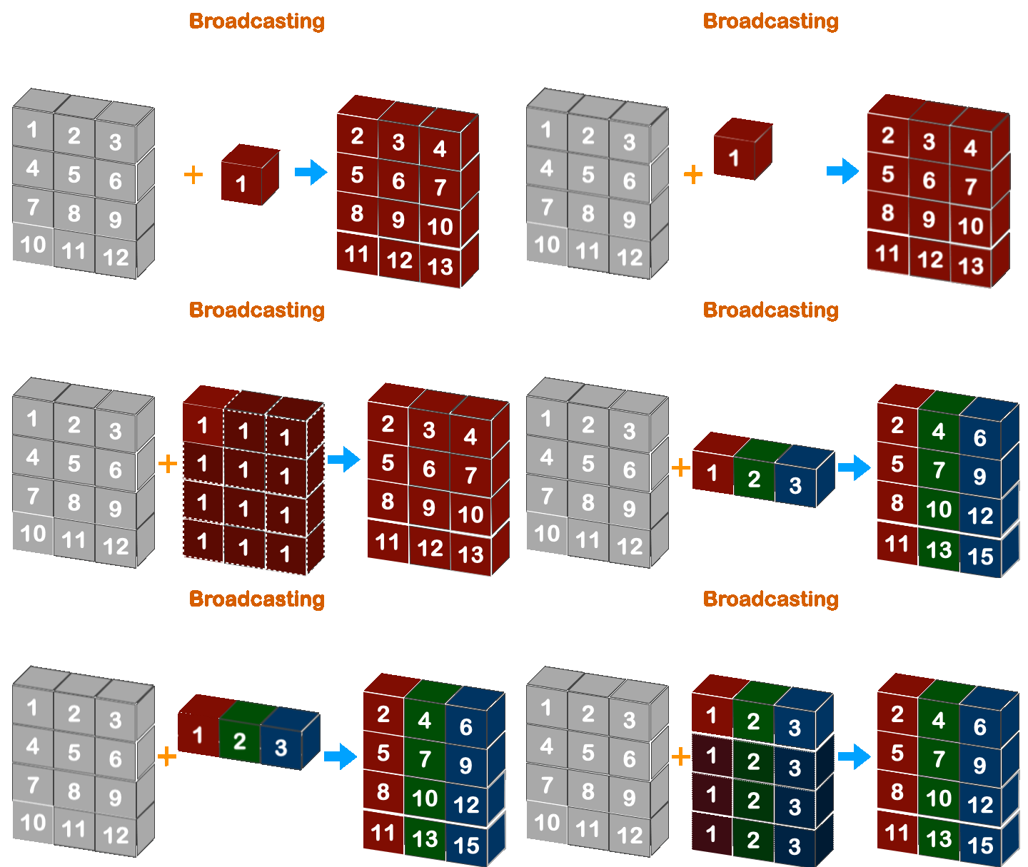
Boradcasting in numpy works when the less dimension is right align with more dimension array.
So, (4, 3) with (3, ) will work, but not with (4, ).
(3, ) -> ([4], 3)
(4, ) -> ([4], 4)
np.broadcast_arrays, broadcast the array to the desired shape. Notice the strides of dc, is (1, 0), because the row axis' element is broadcasted.
da, dc = np.broadcast_arrays(a, c[:, np.newaxis])
print_info(dc)
While nb.broadcast_arrys() take one array as reference and broadcast the other array to the same shape as reference one, we can also manipulate the arr to any shape we want withnp.lib.stride_tricks.as_strided().
def repeat(arr, size):
    return np.lib.stride_tricks.as_strided(
                                arr, shape=(size, ) + (arr.shape),
                                strides = (0, ) + (arr.strides))


print(repeat(b, 5))
print_info(repeat(b, 5))
This function is often used to find the sliding window of the given array.
def sliding_window(arr, win_size):
    sliding_win = np.lib.stride_tricks.as_strided(
                    arr, shape = (arr.shape[0]-win_size+1, win_size),
                    strides = (arr.strides[0], arr.strides[0]))

    return sliding_win


a = np.arange(10, dtype=np.uint8)
print(sliding_window(a, 3))
print(np.mean(sliding_window(a, 3), axis=1))
Let's do something more exciting. We will find the mean of the sliding window. Resulting in the smoother graph. And we will then find mock moving average.
import matplotlib.pyplot as plt
import numpy as np
import altair as alt
import pandas as pd

indexs = np.arange(100)

random_arrays = np.random.normal(0, 0.5, size=100)

# Add some curve to the graph : Sexy, hehe
random_arrays[30:60] += 1

# Let's smooth it out
mean_2 = np.mean(sliding_window(random_arrays, 2), axis=1)
padded_mean_2 = np.pad(mean_2, (1, 0))
mean_5 = np.mean(sliding_window(random_arrays, 5), axis=1)
padded_mean_5 = np.pad(mean_5, (1, 3))
simple_ema = np.array([0.1, 0.15, 0.2, 0.25, 0.3])
ema_size = simple_ema.size
ema = sliding_window(np.pad(random_arrays, (ema_size, ema_size-1), 'reflect'), ema_size) * simple_ema
ema = np.sum(ema, axis=1)[:-5]


df = pd.DataFrame({
    'index':np.hstack((indexs, indexs, indexs, indexs)),
    'values':np.hstack([random_arrays, padded_mean_2, padded_mean_5, ema]),
    'label':[j for j in ['random_arrays', 'mean with 2 neighbour', 'mean with 5 neighbour', 'mock Exponential Moving Average'] for _ in range(100)]
})

# Create a selection that chooses the nearest point & selects based on x-value
nearest = alt.selection(type='single', nearest=True, on='mouseover',
                        fields=['index'], empty='none')

# The basic line
line = alt.Chart(df).mark_line(interpolate='basis').encode(
    x='index:Q',
    y='values:Q',
    color='label:N'
)

# Transparent selectors across the chart. This is what tells us
# the x-value of the cursor
selectors = alt.Chart(df).mark_point().encode(
    x='index:Q',
    opacity=alt.value(0),
).add_selection(
    nearest
)

# Draw points on the line, and highlight based on selection
points = line.mark_point().encode(
    opacity=alt.condition(nearest, alt.value(1), alt.value(0))
)

# Draw text labels near the points, and highlight based on selection
text = line.mark_text(align='left', dx=5, dy=-5).encode(
    text=alt.condition(nearest, 'values:Q', alt.value(' '))
)

# Draw a rule at the location of the selection
rules = alt.Chart(df).mark_rule(color='gray').encode(
    x='index:Q',
).transform_filter(
    nearest
)

# Put the five layers into a chart and bind the data
alt.layer(
    line, selectors, points, rules, text
).properties(
    width=600, height=300
)

# plt.plot(random_arrays, label='origin')
# plt.plot(mean_2, label='mean with 2 neighbour')
# plt.plot(mean_5, label='mean with 5 neighbour')
# plt.plot(ema, label='mock Exponential Moving Average')
# plt.legend()
# plt.show()
Well, as expected, exponentially moving average have some phase shift. It can be corrected with phase shift as described in adam paper. I am too lazy to implement it. hehe

